13  Estimação no Ponto

13.1 Introdução

Um dos esforços da estatística é propor técnicas para estimar caracaterísticas populacionais que auxiliem os tomadores de decisão a fazerem melhores escolhas. Se vamos fazer um programa para treinamento para mulheres desempregadas de baixa renda, precisamos saber qual a taxa de desemprego daquela população e assim propor um número de vagas adequado. Se queremos melhorar o sistema de logística de um entreposto, precisamos entender qual a intensidade de chegada de caminhões nesse entreposto. Se vamos fazer um programa de auxílio para pessoas em situaçao de extrema pobreza, precisamos saber quantas pessoas vivem nessa situação nessa localidade.

Notamos que para a maior parte das questões que temos sobre o mundo, raramente sabemos o que acontece na população. Temos que tentar construir um modelo que nos ajude nessa tarefa e nos de a segurança que as nossas estimativas da realidade sejam boas. Na inferência estatística existem dois objetivos principais.

1. Estimação de parâmetros: valores populacionais

2. Testes de hipótese sobre os parâmetros

Nosso objetivo aqui é estudar técnicas que nos permita avaliar se uma proposta de estimativa de uma caractaristica da população é “boa” e aprender técnicas para encontrar “boas” estimativas. Assim temos duas questões básicas surgem:

1. Quais as características que um “bom” estimador possui?

2. Como decidiremos que uma boa estimativa é “melhor” que outras?

Para saber se uma estimativa é boa ou não vamos introduzir duas ideias aqui, exatidão e precisão.

Dois conceitos importantes:

1. Exatidão: proximidade de cada observação do valor do centro do alvo (nosso caso: parâmetro)

2. Precisão: proximidade de cada observação em relação ao ponto médio de todas, variância.

A figura abaixo traz esses dois conceitos¹:

Figure 13.1: Exatidão e precisão

Uma outra forma de vermos o mesmo conceito é pelo exmplo clássico dos alvos. Vejamos a figura abaixo:

Figure 13.2: Alvo e os conceitos de Exatidão e precisão

Cada x no alvo representa uma tentativa sua de estimar o parâmetro de uma população que é o centro do alvo. A ideia seria que uma boa “arma” (arma aqui é a sua equação matemática) é aquela que acerta ao redor do centro do alvo e menos espelhado possível. Vejamos cada um desses alvos:

1. A: Exato (média das tentativas está no centro do alvo.) Pouco Preciso (observações muito dispersas)

2. B: Pouco Exato e Pouco Preciso

3. C: Exato e Preciso

4. D: Pouco Exato e Muito Preciso

Portanto, notamos que a melhor arma, ou seja, a melhor forma de estimar é pela “arma” C.

13.2 Estimadores e Estimação

Considere uma amostra \((X_1, ..., X_n)\) de uma variável aleatória \(X\), sendo \(X_i\) variáveis aleatíras com a mesma distribuição de \(X\) e \(x_i\) os valores observados. Considere \(\Theta\) um parâmetro populacional, podendo ser por exemplo: \(\mu\) ou \(\sigma\).

NoteDEFINIÇÃO

Um estimador \(T\) do parâmetro \(\Theta\) é qualquer função das observações da amostra, tal que:

Portanto, cada estimador é uma estatística a qual associamos a um parâmetro. Assim temos uma segunda definição:

NoteDEFINIÇÃO

Uma Estimativa é o valor \(t\) que somente depende da amostra observada \(x_1, x_2, ..., x_n\). Ou seja, é uma função somento do banco de dados coletado:

Veja a situação apresentada abaixo. Sabe-se que temos o retorno de uma carteira dada por \(X\) que é uma variável aleatória. Sabe-se que a esperança do rerotno dessa carteira (\(\mathbb{E}(X)\)) que chamaremos de \(\Theta\) é de 0. Encontramos duas maneiras de estimar esse retorno. Abaixo temos a distribuição de dois estimadores \(T_1\) e \(T_2\) do parâmetro \(\Theta\).

#Distribuição de dois estimadores, T1 e T2,  para o parâmetro populacional
x<-seq(-5,7,0.1) 
T1<-dnorm(x = x, mean = 3, sd=1)   
T2<-dnorm(x = x, mean = 0, sd=1)

plot(x,T1,xlab="ti",type="l",main=NULL, col="steelblue3",lwd=2, ylab="f(ti)",
     xaxt="n",cex.axis=0.65, cex.lab=0.8 ) 
abline(v=0, col="black", lty=2)
par(new=TRUE)
plot(x,T2,xlab="", ylab="",type="l",col="wheat4",lwd=2,xaxt="n",
     cex.axis=0.65, cex.lab=0.8 ) 
axis(1,at=c(0),labels =c(expression(Theta)),cex.axis=0.65, cex.lab=0.8) 
legend("topleft", legend=c("T1", "T2"),col=c("steelblue3", "wheat4"), 
       lty=1:1, box.lty=0,cex=0.8)

Função Distribuição de Probabilidade Normal e Função Distribuição Acumulada Normal

Questão

Definir uma função \(T_i= h(X_1, ..., X_n)\) que seja próxima de \(\Theta\) segundo algum critério. Ou seja, que acerte em média o parâmetro e que não seja muito dispersa!

13.3 Propriedades dos Estimadores

13.3.1 Tendenciosidade ou Viés

Suponha que estamos querendo estudar o desempenho dos alunos na Prova do ENEM, \(X\), que vamos assumir que tenha distribuição normal com \(\mathbb{E}(X)=2000\) e \(\sigma=400\). Vamos observar 50 alunos que fizeram a prova em 2019 e estimar a esperança da nota utilizando a fórmula \(\bar{X}\). Iremos repetir o processo de amostragem 100.000 vezes. Assim, vamos coletar 50 pessoas e fazer a média para essa amostragem, \(\bar{X}_{50}\) e repetimos esse processo 100 mil vezes. Teremos portanto 100 mil médias. Vejamos a distribuição dessas médias feitas no R:

# Distribuição da nota dos alunos que fizeram ENEM, X. 
x_normal<-rnorm(10000,mean=2000, sd= 400)

#Amostragem:
# Criando os vetores numéricos 
xbar50<-numeric()
var_amostral50<-numeric()
# Extraindo 100 mil amostras de 50 alunos e fazendo a média para cada uma. 
# Teremos 100.000 médias  
for ( i in 1:100000){
  smp<-sample(x_normal,replace = TRUE,size = 50)
  xbar50[i]<-mean(x_normal[smp])
}

# Plotando as médias obtidas
hist(xbar50, col="steelblue3",freq = FALSE, breaks = 25,main="",
     xlim=c(1800, 2200), ylab="Dist. da média", xlab="médias para n=50",
     xaxt="n",border="steelblue3")
abline(v=2000, col="black", lty=2)
text(2000, 0.0003, expression(Theta))
axis(1,at=c(1800, mean(xbar50), 2200),labels =c(1800, round(mean(xbar50)),
    2200),cex.axis=0.65, cex.lab=0.8) 

Distribuição do estimador da Esperança da Nota do ENEM

Observa-se que neste caso o valor númerico central representa \(\mathbb{E}(\bar{X})\) e a linha pontilhada mostra \(\mathbb{E}(X)=2000=\Theta\). Ainda pode-se observar que encontramos diversos valores para \(\bar{X}\), variando de 1800 a 2200, mas com grande concentração ao redor de 2000.

Com base na figura 3 que apresenta dois estimadores e na figura 4 que mostra o resultado para uma estimativa da Esperança, temos a seguinte definição:

NoteDEFINIÇÃO

O estimador \(T\) é chamado de estimador não-viesado, ou não-tendencioso, para o parâmetro \(\Theta\) se:

\(\mathbb{E}(T)=\Theta\) para todo \(\Theta\)

Independente do valor de \(\Theta\), sendo a diferença \(\mathbb{E}(T)-\Theta\) chamada de viés de \(T\). Se a diferença é diferente de 0, T é viesado.

13.3.1.1 Estimadores não viesados para Esperança e Variância populacional.

Considere uma população com N elementos e com a esperança populacional de uma população de tamanho N:

\[\mu =\frac{1}{N}\sum_{j=1}^{N}X_j\]

Um bom estimador para a Esperança populacional seria a média, “copiando” a formulação populacional e consierando \(n\) o tamanho da amostra, ou seja:

\[\bar{X} =\frac{1}{n}\sum_{i=1}^{n}X_i\]

Observe que ele é um estimador não visesado pois

\[\mathbb{E}(\bar{X})=\frac{1}{n}\mathbb{E}[X_1+X_2+...+X_n]\]

\[\mathbb{E}(\bar{X})=\frac{1}{n}[\mathbb{E}(X_1)+\mathbb{E}(X_2)+...+\mathbb{E}(X_n)]\]

\[\mathbb{E}(\bar{X})=\frac{1}{n}[\mu+\mu+...+\mu]=\frac{1}{n}n\mu=\mu\]

Da mesma forma podemos utilizar o princípio de “copiar” para achar um estimador (\(\hat{\sigma}^2\)) para a variância populacional \(\sigma^2\), assim:

\[\sigma^{2}=\frac{1}{N}\sum_{i=1}^{N}(X_i - \mu)^{2} \]

E um possível estimador para \(\sigma^{2}\) (observe que colocamos um chapéu sobre \(sigma\)) será:

\[\hat{\sigma}^{2}=\frac{1}{n}\sum_{i=1}^{n}(X_i - \overline{X})^{2} \]

Entretanto, tal estimador é viesado pois:

\[\sum_{i=1}^{N}(X_i - \overline{X})^{2} = \sum_{i=1}^{N}(X_i - \mu + \mu - \overline{X})^{2}=\sum_{i=1}^{N}((X_i - \mu)- (\overline{X}-\mu))^{2}\]

\[= \sum_{i=1}^{N}(X_i - \mu)^{2} - 2 \sum_{i=1}^{N}(X_i - \mu) (\overline{X} - \mu) + \sum_{i=1}^{N}(\overline{X} - \mu)^{2}\]

Note que \((\overline{X} - \mu)\) é constante. Então dado que:

\[\sum_{i=1}^{N}(X_i - \mu)= \sum_{i=1}^{N}X_i - n\mu\]

\[\overline{X}=\frac{1}{n}\sum_{i=1}^{N}X_i \]

Temos que:

\[n \overline{X}=\sum_{i=1}^{n}X_i \rightarrow \sum_{i=1}^{n}(X_i - \mu)=n(\overline{X}-\mu)\]

Logo:

\[\begin{equation} \begin{split} \sum_{i=1}^{n}(X_i - \overline{X})^{2} & = \sum_{i=1}^{n}(X_i - \mu + \mu - \overline{X})^{2} \\ & = \sum_{i=1}^{N}(X_i - \mu)^{2} - 2 n (\overline{X} - \mu)^{2} + n(\overline{X} - \mu)^{2} \\ & =\sum_{i=1}^{N}(X_i - \mu)^{2} - n (\overline{X} - \mu)^{2} \end{split} \end{equation}\]

Assim:

\[\begin{array}{ccc} \mathbb{E}(\hat{\sigma}^{2})&=E[\frac{1}{n}\{ \sum_{i=1}^{n}(X_i - \mu)^{2} - n (\overline{X} - \mu)^{2} \}] \\ \\ &=\frac{1}{n}\{ \sum_{i=1}^{n}E (X_i - \mu)^{2} - n E (\overline{X} - \mu)^{2} \} \\ \\ &=\frac{1}{n}\{ \sum_{i=1}^{n}Var(X_i) - n Var(\overline{X}) \} \end{array}\]

Como \(Var(X_i)=\sigma^{2}\) e \(Var(\overline{X})=\sigma^{2}/n\):

\[\begin{array}{ccc} \mathbb{E}(\hat{\sigma}^{2})=\frac{1}{n}\{ \sum_{i=1}^{n} \sigma^{2} - n \frac{ \sigma^{2}}{n} \} \\ \\ = \sigma^{2} - \frac{ \sigma^{2}}{n} \\ \\ =\sigma^{2}\frac{n-1}{n} \end{array}\]

Assim \(\hat{\sigma^{2}}\) é um estimador viesado para o parâmetro \(\sigma^{2}\) e o viés é dado por:

\[V = V(\hat{\sigma^{2}})= E(\hat{\sigma^{2}})-E(\sigma)=-\frac{\sigma^{2}}{n}\]

Como \(V\) é negativo estamos subestimando o verdadeiro valor do parâmetro. Entretanto, o viés diminui com n:

Quando \(n \rightarrow \infty\) temos que \(V \rightarrow 0\)

Para obter o melhor estimador não-viesado do parâmetro \(\sigma^2\) basta considerar

\[\begin{array}{ccc} S^2= \frac{n}{n-1} \hat{\sigma}^2 \\ \\ \therefore \mathbb{E}(\frac{n}{n-1} \hat{\sigma}^2)=\frac{n}{n-1} \mathbb{E}(\hat{\sigma}^2)=\frac{n}{n-1}\frac{n-1}{n} \sigma^2=\sigma^2 \end{array}\]

Definimos: \[\begin{array}{ccc} S^2= \frac{n}{n-1} \hat{\sigma}^2 = \frac{n}{n-1}\frac{1}{n} \sum_{i=1}^{n}(X_i - \overline{X})^2 \\ \\ S^2=\frac{1}{n-1}\sum_{i=1}^{n}(X_i - \overline{X})^2 \end{array}\]

Onde:

\[E(S^2)=\sigma^2\]

\(S^2\) é um estimador não-viesado

13.3.2 Eficiência

Agora temos a seguinte situação, dado dois estimadores não viesados, como escolher qual dos dois seria melhor? Vejamos a situação abaixo:

# Vamos estudar a nota do ENEM. 
x_normal<-rnorm(10000,mean=2000, sd= 400)

# Criando os vetores numéricos 
xbar50<-numeric()
med50<-numeric()
# Extraindo duas mil amostras de 15 e fazendo a média e 
# variância. Teremos 2000 médias e 2000 variâncias 
for ( i in 1:100000){
  smp<-sample(x_normal,replace = TRUE, size = 50)
  xbar50[i]<-mean(x_normal[smp])
  med50[i]<-median(x_normal[smp])
}
par(mfrow=c(1,2))
hist(xbar50, col="steelblue3",freq = FALSE, breaks = 25,main="",
     xlim=c(1800, 2200), ylab="Densidade", xlab="Média para n=50",xaxt="n",
     border="steelblue3")
abline(v=2000, col="black", lty=2)
axis(1,at=c(1800, mean(xbar50), 2200),labels =c(1800, round(mean(xbar50)),
    2200),cex.axis=0.65) 
text(2000, 0.0003, expression(Theta))
hist(med50, col="steelblue3",freq = FALSE, breaks = 25,main="",
     xlim=c(1800, 2200), ylab="Densidade", xlab="Médiana para n=50",xaxt="n",
     border="steelblue3")
abline(v=2000, col="black", lty=2)
axis(1,at=c(1800, mean(xbar50), 2200),labels =c(1800, round(mean(xbar50)),
    2200),cex.axis=0.65) 
text(2000, 0.0003, expression(Theta))

Distribuição de dois estimadores não viesádos para a Esperança da População , média e mediana

A figura 5 mostra a distribuição de dois estimadores da esperança populacional das notas do ENEN, a média e a mediana. Observa-se que elas não são viesadas. Qual das duas seria a melhor? Poderia utilizar as duas?

Visualmente notamos que a precisão do gráfico do estimador que utiliza a mediana amostral é maior do que a do gráfico do estimador que uriliza a méia amostral. Matematicamente temos o seguinte:

\[Var(\hat{md})=\pi \frac{\sigma^2}{n}>\frac{\sigma^2}{n}= Var(\bar{X})\]

\(\bar{X}\) tem menor variância e é melhor a partir deste critério. Assim, a média acerta o alvo como a mediana, entretanto a dispersão é menor para média, ou seja, maior precisão. O estimador da esperança que utiliza a média é exato e mais preciso do que o estimador que utiliza a mediana e portanto é preferível!

Em termos práticos, estimadores mais precisos ou eficientes, geram estimativas que tem maior chance de estarem perto do verdadeiro parâmetro. Veja o gráfico que para a média a chance de obtermos valores ao redor de 2.200 é muito baixo e apresenta-se maior na mediana.

NoteDEFINIÇÃO

Sejam \(T_1\) e \(T_2\) são dois estimadores não-viesados de um mesmo parâmetro \(\Theta\). Dizemos que \(T_1\) é mais eficiente do que o estimador \(T_2\) se

13.3.3 Erro quadrático médio

A performance de um estimador deve ser avaliada principalmente pela maneira que se dispersa ao redor do parâmetro \(\Theta\) a ser estimado. Considere o erro amostral:

Esse é o erro que cometemos ao estimar o parâmetro \(\Theta\) da distribuição da v.a. \(X\) pelo estimador \(T\) baseado em uma amostra

NoteDEFINIÇÃO

Sendo \(T\) o estimador do parâmetro populacional \(\Theta\), então o Erro Quadrático Médio (EQM) do estimador \(T\) será:

\[EQM(T;\Theta) = E(e^{2})= E(T-\Theta)^{2}\]

---

Desenvolvendo:

\[\begin{array}{ll} EQM(T;\Theta) &= E(e^{2})=E(T-\Theta)^{2} \\ \\ &= E(T-E(T))^{2}+ E(E(T)-\Theta)^{2} \\ \\ &= Var (T) + V^{2} \end{array}\]

Sendo \(Var (T)\) a variância do estimador e \(V^{2}\) o viés ao quadrado. Dessa forma, se conseguirmos encontrar o estimador que possui o menor EQM, esse será o estimador que reduz viés e variância. Muitas vezes buscamos em uma família de estimadores consistentes aqueles que possuem o menor EQM.

O gráfico apresenta o EQM da média e da mediana ao estimar a esperança da nota do ENEM. Observe que o EQM da mediana é maior, distribuição com mais peso a direita, ou seja, a chance de erros maiores é maior ao utilizar a mediana como estimador. Por isso preferimos a média.

# Vamos estudar a nota do ENEM. 
x_normal<-rnorm(10000,mean=2000, sd= 400)

# Criando os vetores numéricos 
xbar50<-numeric()
med50<-numeric()
e50<-numeric()
e50md<-numeric()
# Extraindo duas mil amostras de 15 e fazendo a média e 
# variância. Teremos 2000 médias e 2000 variâncias 
for ( i in 1:100000){
  smp<-sample(x_normal,replace = TRUE,size = 50)
  xbar50[i]<-mean(x_normal[smp])
  e50[i]<-(xbar50[i]-2000)^2
  med50[i]<-median(x_normal[smp])
  e50md[i]<-(med50[i]-2000)^2
}

hist(e50md, col="wheat4",freq = FALSE, breaks = 120,main="",
     xlim=c(0, 15000), ylab="Densidade do EQM", xlab="EQM",
     border="wheat4")

par(new=TRUE)
hist(e50, col="steelblue3",freq = FALSE, breaks = 120,main="",xaxt="n",
     yaxt="n", xlim=c(0, 15000), ylab="Densidade do EQM", xlab="EQM",
     border="steelblue3")
legend("topright", legend=c("EQM- mediana", "EQM - média"),col=c("wheat4",
      "steelblue3"), lty=1:1, box.lty=0,cex=0.8)

Erro Quadrático Médio de dois estimadores não viesádos para a Esperança da População , média e mediana

13.3.4 Consistência

A consistência é uma propriedade que surge quando o tamanho amostral cresce, ou seja, quando \(n\rightarrow \infty\). Essa é uma propriedade importante para um estimador, pois deve convergir para o verdadeiro parâmetro quando a quantidade de informação aumenta, ou seja, maior tamanho amostral.

Podemos calcular \(\overline{X}\) para diversos tamanho de amostra, obtemos uma sequência de estimadores \(\overline{X}_n\) para n=1,2,…. Quando \(n\) cresce e a distribuição de \(\overline{X}_n\) torna-se mais concentrada ao redor da média real \(\mu\). Dessa forma, \(\overline{X}_n\) é uma sequência consistende de estimadores de \(\mu\).

Veja o gráfico abaixo para amostra de tamanho 50, 500 e 1500.

# Voltamos a nota do ENEM. 
x_normal<-rnorm(10000,mean=2000, sd= 400)
# Criando os vetores numéricos 
xbar50<-numeric()
xbar500<-numeric()
xbar1500<-numeric()
# Extraindo duas mil amostras de 15 e fazendo a média e 
# variância. Teremos 2000 médias e 2000 variâncias 
for ( i in 1:50000){
  smp<-sample(x_normal,replace = TRUE, size = 50)
  xbar50[i]<-mean(x_normal[smp])
  smp1<-sample(x_normal,replace = TRUE,size = 500)
  xbar500[i]<-mean(x_normal[smp1])
  smp2<-sample(x_normal,replace = TRUE,size = 1500)
  xbar1500[i]<-mean(x_normal[smp2])
}
hist(xbar50, col="wheat4",freq = FALSE, breaks = 25,main="",
     xlim=c(1800, 2200), ylab="Densidade da Média", xlab="Média de X", 
     border="wheat4")
par(new=TRUE)
hist(xbar500, col="steelblue3",freq = FALSE, breaks = 25,main="",xaxt="n",
     yaxt="n", xlim=c(1800, 2200), ylab="", xlab="", border="steelblue3")
par(new=TRUE)
hist(xbar1500, col="gray",freq = FALSE, breaks = 25,main="",xaxt="n",
     yaxt="n", xlim=c(1800, 2200), ylab="", xlab="",border="gray")
text(2000, 0.0008, expression(mu))
legend("topright", legend=c("Amostra","n=50","n=500","n=1500"),col=c("white", 
      "wheat4","steelblue3","gray"), lty=1:1, box.lty=0,cex=0.8)

Consistência do estimador não viesados para a Esperança da População , média

Observe que ao aumentar o tamanho amostral a distribuição vai se concentrando ao redor do parâmetro populacional. Ou seja, \(\bar{X}\) é consistente. Assim tem-se a seguinte definição:

NoteDEFINIÇÃO

Uma sequência \(\{T_n \}\) de estimadores de um parâmetro \(\Theta\) é consistente se para todo \(\varepsilon >0\):

\[P\{ | T_n - \Theta | > \varepsilon \} \rightarrow 0 , n \rightarrow \infty\]

Para o caso específico da média \(\bar{X}\), tem-se:

\[P\{ | \bar{X} - \mu | > \varepsilon \} \rightarrow 0 , n \rightarrow \infty\]

Dessa forma temos o seguinte Teorema:

NoteTEOREMA

Considerando a desigualdade de Tchebycheff, tem-se:

\[P\{ | T_n - \Theta | < \varepsilon \} \geq 1-\frac{\sigma^2}{\varepsilon^2n}\]

Dessa forma sequência \(\{T_n \}\) de estimadores de um parâmetro \(\Theta\) é consistente se:

\[lim_{n \rightarrow \infty} P\{ | T_n - \Theta | < \varepsilon \} = 1\]

Podemos ainda escrever:

A prova desse teorema foi vista na seção anterior quando apresentamos a Lei dos Grandes Números. Uma maneira mais direta para testar a consistência do estimador pode-se utilizar o seguinte resultado:

Proposição

Uma sequência \(\{T_n \}\) de estimadores de um parâmetro \(\Theta\) é consistente se:

\[lim_{n \rightarrow \infty} E(T_n) = \Theta\]

\[lim_{n \rightarrow \infty} Var (T_n) = 0\]

TipEXEMPLO

Seja \(S^{2}\) um estimador não viesado, sendo, \(E(S^{2})=\sigma^{2}\). Se X tiver uma distribuição Normal ~\(N(\mu,\sigma^{2})\) e \(X_1, ..., X_n\) as \(n\) medições de \(X\), então:

\[Var(S^{2})=\frac{2 \sigma^{4}}{n-1}\]

e

\[lim_{n \rightarrow \infty}Var(S^{2})=0\]

Portanto, \(S^{2}\) é um estimador consistente pois:

TipEXEMPLO

Para o caso do estimador incosistente \(\hat{\sigma^2}\) da variância populacional onde \(\mathbb{E}(\hat{\sigma^2})=\sigma^2-\frac{\sigma^2}{n}\), tem-se:

\[\begin{array}{ccc} \mathbb{E}(\hat{\sigma^{2}})=\hat{\sigma^{2}}- \frac{\hat{\sigma^{2}}}{n} \Rightarrow lim_{n \rightarrow \infty} \mathbb{E}(\hat{\sigma^{2}})={\sigma^{2}} \end{array}\]

\[\begin{array}{ccc} Var(\hat{\sigma^{2}})= (\frac{n-1}{n})^{2} Var(S^{2}) = \frac{(n-1)^2}{n^{2}} \frac{2\sigma^{4}}{n-1}=\frac{n-1}{n^{2}} 2 \sigma^{4} \Rightarrow lim_{n \rightarrow \infty} Var(\hat{\sigma^{2}})=0 \end{array}\]

Portanto, \(\hat{\sigma^{2}}\) é um estimador consistente

Esse resultado mostra o porque muitas vezes utilizamos os dois estimadores para estimar a variância populacional, pois para um \(n\) grande ambos são consistentes. Além disso, a variância de \(\hat{\sigma}^2\) é menor.

13.4 Métodos de Estimação

Até agora “imitamos” o que acontece na população para a amostra com os estimadores \(\overline{X}\) e \(S^2\). Entretanto podemos ter modelos mais complexos e parâmetros populacionais que não conseguimos imitar o que acontece na população.

Vamos considerar que gostariamos de compreender os determinantes da renda de uma pessoa. Afinal, renda significa consumo e bem estar e gostariamos de saber porque tem pessoas que ganham mais e pessoas que ganham menos. Assim poderemos propor políticas públicas que sejam mais efetivas.

Com o passar do tempo e vários estudos os economistas perceberam que a educação é um fator importante para compreender a renda das pessoas.

Ou seja, o salário é uma função da educação que recebemos. Veja o gráfico 1 abaixo entre o ln do PIB per capita e os anos médios de educação em diversos países do mundo².

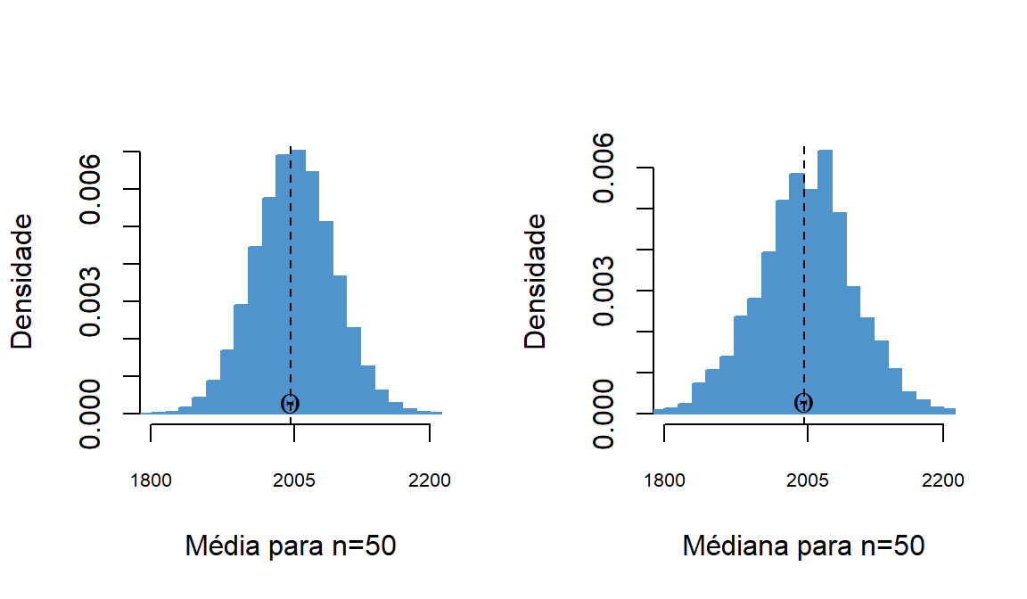
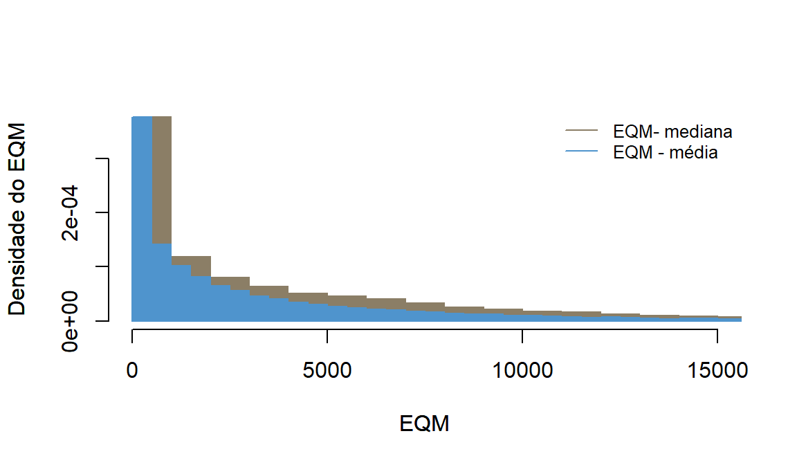
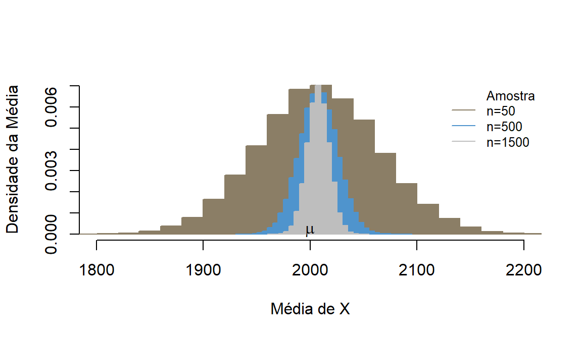
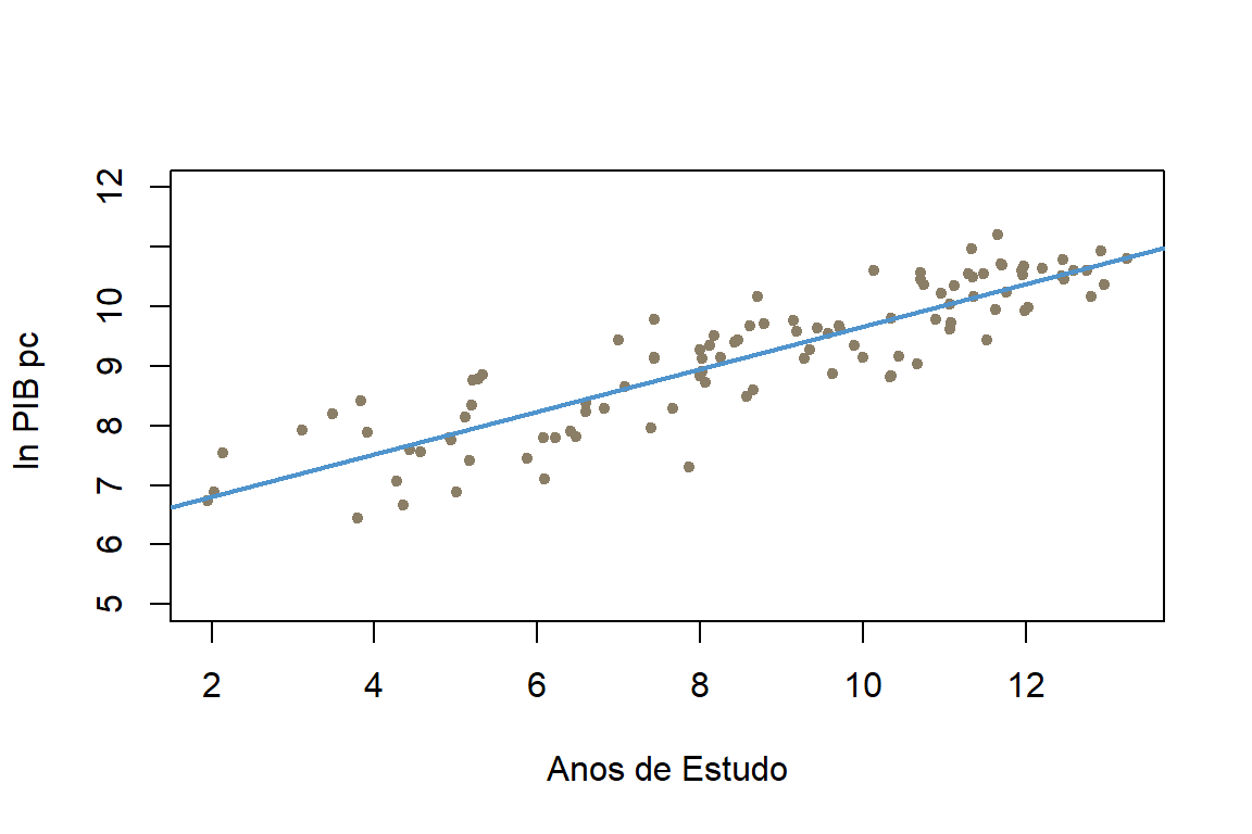
#Pib per capita em ln e anos de estudos de diversos países em 2010
ln_salario<- c(9.16, 9.44, 9.67, 10.71, 10.61, 7.79, 9.55, 10.55, 8.87, 7.56,
               8.48, 9.51, 9.61, 7.75, 7.90, 10.60, 9.80, 9.14, 9.27, 9.40, 
               7.80, 10.24, 10.17, 6.45, 10.68, 9.35, 9.12, 9.12, 8.72, 8.84,                   10.56, 10.49, 7.89, 10.61, 8.28, 10.16, 8.76, 7.41, 8.24, 10.64, 
               9.93, 10.54, 8.38, 8.90, 9.76, 9.14, 10.78, 10.46, 8.81, 10.51,
               9.14, 7.82,  7.80, 6.67, 10.97, 6.88, 9.79, 7.54, 10.04, 9.63,
               9.58, 8.77, 6.88, 8.14, 7.60, 10.69, 10.34, 8.29, 6.74, 11.20,
               8.34, 9.62, 8.83, 9.13, 8.59, 9.95, 10.16, 9.73, 9.99, 7.92,
               9.43, 7.06, 9.34, 10.36, 10.36, 9.03, 8.19, 8.86, 10.61, 10.93,
               8.65, 10.52, 9.43, 7.11, 10.22, 9.27, 9.79, 7.45, 10.46, 10.81,
               9.67, 9.70, 8.42, 7.96, 7.30)

educa<- c(10.44, 7, 9.71, 11.69, 10.13, 6.22, 9.57, 11.29, 9.63, 4.57, 8.57,
          8.17, 11.07, 4.94, 6.41, 12.74, 10.35, 8.25, 9.35, 8.43, 4.93, 11.76,
          12.8, 3.79, 11.97, 8.12, 8.02, 7.44, 8.06, 10.35, 10.71, 11.34, 3.92,
          12.58, 7.66, 11.36, 5.21, 5.17, 6.6, 12.2, 11.98, 11.48, 6.59, 8.02,
          9.15, 7.43, 12.45, 10.71, 10.33, 12.44, 10, 6.47, 6.08, 4.35, 11.33,
          5.01, 10.89, 2.14, 11.06, 9.44, 9.18, 5.27, 2.03, 5.11, 4.44, 11.71,
          11.12, 6.82, 1.95, 11.65, 5.19, 9.72, 7.99, 9.28, 8.65, 11.62, 8.71,
          11.08, 12.02, 3.11, 11.52, 4.28, 9.89, 12.96, 10.75, 10.67, 3.49,
          5.33, 11.95, 12.92, 7.07, 11.96, 8.47, 6.09, 10.96, 8, 7.44, 5.87,
          12.46, 13.24, 8.61, 8.78, 3.84, 7.4, 7.86)  

bd = data.frame(ln_salario, educa)

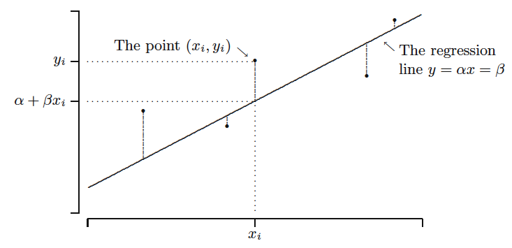
plot(bd$educa, bd$ln_salario, xlab="Anos de Estudo", 
     ylab="ln PIB pc ", pch=20, col="wheat4",ylim=c(5,12))
abline(lm(bd$ln_salario~bd$educa), col="steelblue3", lwd = 2)

Anos de estudos e ln do PIB pc de diversos países em 2010

Observe que existe uma relação ascendente, ou seja, quanto maior a educação maior renda per capita. Entretanto, observa-se também uma imprecisão, ou algum componente aleatório que não nos permite determinar precisamente a renda dada a escolaridade. Para países com 10 anos de estudos as rendas variam mais ou menos entre 8,5 e 10,5. Dessa forma um possível modelo para tratarmos essa problema seria:

A questão é qual a função que descreveria essa relação entre escolaridade de rend? O que podemos assumir é que h é uma função crescente e parece razoável que possamos assumir uma função linear como representada pela linha vermelha. Podemos dizer que existe uma correlação entre renda e educação, ou seja, uma dependência linear. Um possível e mais comum modelo seria uma função linear que relaciona renda e educação e que considere as flutuações, ou seja:

\[Renda=\alpha+\beta . Educação + u_i\]

Essa é a linha de regressão sendo que \(\alpha\) e \(\beta\) parâmetros populacionais. O parâmetro \(\beta\) representa a influência de um ano a mais de educação sobre a renda per capita e sendo \(\mathbb{E}(u_i)=0\) para \(i=1,...n\)

O que precisamos estimar é o parâmetro populacional \(\beta\). Assim, deve existir uma estimador \(\hat{\beta}=h(Y_i,X_j)\) que nos permitir estimar quanto que cada a ano a mais de educação poderia nos trazer a mais de renda. Diferentemente do que fizemos para Esperança, agora temos pouco ou nenhuma intuição do que seria a formulação de \(h\).

Existem algumas maneiras para fazermos isso:

1. Estimadores de Momentos

2. Estimadores de Máxima Verossimilhança

3. Mínimos Quadrados

Veremos duas delas Minimos Quadrados e Máxmia Verossimilhança.

13.4.1 Estimadores de Mínimos Quadrados

Iremos continuar como nosso exemplo anterior onde gostariamos de saber como cada ano a mais de educação poderia afetar a renda per capita. Primeiramente vamos considerar o gráfico anterior mas de uma forma mais didática. Considere a figura 2³:

Figure 13.3: Valores observados e estimados para y

Temos que observar dois pontos importantes, o primeiro é que os pontos representam valores do par ordenado \((x_i,y_i)\). A linha representa os valores estimados ou projetados de \(Y\) para dado valor de \(X\), ou seja, \(\hat{y}_i=\alpha+\beta.x_i\). Um bom estimador, ou seja, um bom \(\alpha\) e \(\beta\), deveria ser aquele que torne o menor possível essa distância entre observado \(y_i\) e estimado\(\hat{y_i}\), ou seja, minimiza o erro que cometemos ao tentar estimar o valor observado. Nesse sentido, deve minimizar conjuntamente a distância dos pontos (observado) até a linha (estimado). Dessa forma, os erros podem ser assim descritos:

\[e=(y_i-\hat{y}_i)=(y_i-\alpha-\beta.x_i)\]

Como não é importante se os erros são positivos ou negativos, utilizamos aqui a minimização da soma dos erros ao quadrado. Para verem uma simulação sobre esse ajustamento ou minimização dos erros ao qudrado, acesse “https://phet.colorado.edu/en/simulation/least-squares-regression”. Portanto devemos minimizar:

\[S(\alpha, \beta)=\sum_{i=1}^{n}(y_i-\hat{y}_i)^2=\sum_{i=1}^{n}(y_i-\alpha-\beta.x_i)^2\]

Podemos entender essa minimização como o procedimento para encontrar os estimadores \(\hat{\alpha}\) e \(\hat{\beta}\) que gerem o menor erro quadrático médio. Ou seja, encontraremos os estimadores lineares que reduzem viés e variância.

Minimizando os erros ao quadrado e utilizando a regra da cadeia (considere \(z=y_i-\alpha-\beta.x_i\)):

\[\begin{array}{clc} S(\alpha, \beta)=&\sum_{i=1}^{n}(y_i-\alpha-\beta.x_i)^2 \\ \\ \frac{\partial S(\alpha, \beta)}{\partial \alpha} =& 2\sum (y_i -\hat{\alpha}- \hat{\beta} x_i)(-1)=0 \\ \\ 0=& -\sum y_i+n\hat{\alpha}+\hat{\beta}\sum x_i \\ \\ \hat{\alpha}=&\frac{\sum y_i-\hat{\beta}\sum x_i}{n} \\ \\ \hat{\alpha}=&\bar{y}-\hat{\beta}\bar{x} \end{array}\]

Agora derivando em relação a \(\beta\):

\[\begin{array}{rlc} \frac{\partial S(\alpha, \beta)}{\partial \beta} =& 2\sum (y_i -\hat{\alpha}- \hat{\beta} x_i)(-x_i)=0 \\ \\ 0=& -2\sum y_i x_i + 2\sum (x_i \bar{y}-x_i\hat{\beta}\bar{x})+2\hat{\beta}\sum x_i^2 \\ \\ 0=& -2\sum y_i x_i + 2\bar{y}\sum x_i -2\hat{\beta}\bar{x}\sum x_i+2\hat{\beta}\sum x_i^2 \\ \\ 2\hat{\beta}(\sum x_i^2-\frac{\sum x_i}{n}\sum x_i) =& 2(\sum y_i x_i - \frac{\sum y_i}{n}\sum x_i) \\ \\ \hat{\beta}(\frac{n\sum x_i^2-(\sum x_i)^2}{n}) =& \frac{n\sum y_i x_i - \sum y_i\sum x_i}{n} \\ \\ \hat{\beta}=&\frac{n\sum y_i x_i - \sum y_i\sum x_i} {n\sum x_i^2-(\sum x_i)^2} \end{array}\]

Podemos reescrever a equação acima como:

\[\begin{array}{rlc} \hat{\beta}=&\frac{n\sum y_i x_i - \sum y_i\sum x_i} {n\sum x_i^2-(\sum x_i)^2}= \frac{\sum (x_i - \bar{x})(\sum y_i-\bar{y})}{\sum (x_i-\bar{x})^2}= \frac{\sum y_i x_i - n\bar{y}\bar{x}} {\sum x_i^2-n\bar{x}^2} \end{array}\]

Dessa forma temos dois estimadores, do intercepto, \(\hat{\alpha}\) e da inclinação \(\hat{\beta}\) e eles representam os estimadores de mínimos qudrados para o modelo de regressão que estavamos discutindo!

Esse é o modelo padrão que iremos estudar em econometria. Entretanto, para fins didáticos podemos utilizar o modelo sem intercepto (ou em casos muito especiais em econometria), o princípio é o mesmo de minimização dos erros ao quadrado conforme derivação abaixo:

Resolvendo temos que:

\[\begin{array}{rlc} S( \beta)=&\sum_{i=1}^{n}(y_i-\beta.x_i)^2 \\ \\ \frac{\partial S( \beta)}{\partial \beta} =& 2\sum (y_i - \hat{\beta} x_i)(-x_i)=0 \\ \\ 0 =& 2(-\sum x_iy_i + \sum \hat{\beta} x_i^2) \\ \\ \hat{\beta} \sum x_i^2 =& \sum x_iy_i \\ \\ \hat{\beta}_{MQ}=&\frac{\sum x_iy_i}{\sum x_i^2 } \end{array}\]

Vamos utilizar os nossos dados apresentados acima e calcular no R o resultado. Faremos na força bruta e utilizando a rotina do programa. Veja abaixo:

# Fazendo na mão. Usando a equação que derivamos acima
B<-((sum(educa*ln_salario)-105*(mean(educa)*mean(ln_salario))))/
  ((sum(educa^2)-105*(mean(educa)^2)))
A<-mean(ln_salario-B*mean(educa))
B

[1] 0.3568401

A

[1] 6.092204

# Usando a rotina do R para Mínimos Quadrados
reg<-lm(ln_salario~educa)
reg

Call:
lm(formula = ln_salario ~ educa)

Coefficients:
(Intercept)        educa  
     6.0922       0.3568  

Observe que cada ano a mais de educação que um pais consegue, aumenta em 0.357 o ln da renda per capita. Mostrando que renda e educaçao estão correlacionado! Dessa forma, nossa equação para achar \(\hat{Y}\) será:

\[\hat{Y}=\hat{\alpha}+\hat{\beta}x\] ou seja,

\[\hat{Y}=6.092+0.357x\]

Dessa forma um país que consiga atingir 10 anos de média de educação terá o ln da renda estimado em \(9.66\). Isso pode ser visto no gráfico acima. Um outro ponto que será estudo em econometria e a interpretação do coeficiente. Aqui somente deixamos a interpretação desse coeficiente e não entramos no detalhe da sua explicação. Como é um modelo com \(Y\) em ln e \(x\) em nível, modelo log-linear, deveremos fazer \(exp(0.35)=1,43\), isso implica que cada aumento de 1 ano de escolaridade média da população aumenta da renda do país em 43%. Importante que cada modelo, log-log, log-linear e linear-linear tem sua própria maneira de interpretar o coeficiente.

13.4.2 Estimador de Máxima Verossimilhança

13.4.2.1 Intuição:

Suponha que gostaríamos de saber qual seria uma boa estimativa da esperança da nota do IDEB nos município brasileiros para os primeiros anos do fundamental em 2017. Vamos coletar 500 municipios e vamos plotar o histograma conforme figura 3 abaixo.

# Distribuição da nota dos alunos que fizeram ENEM, X. 
smp<-sample(rnorm(5500,mean=5.6, sd= 1.0139),replace = TRUE,size = 500)

# Plotando as médias obtidas
hist(smp, col="steelblue3",freq = FALSE, breaks = 25,main="",
     xlim=c(0, 10), ylab="Dist. das notas IDEB", xlab="notas IDEB ",
     border="steelblue3")

Distribuição da amostra das notas do IDEB 2017, para os primeiros anos do fundamental de 500 municípios

Esse são os dados que observamos, ou seja, uma amostra de 500 elementos onde temos \(X_1, X_2,...,X_{500}\) as 500 medições sendo que todas elas tem a mesma distribuição de e igual a de \(X\), \(f(x;\mu)\). O gráfico acima apresenta os valores observados das medições, \(x_1,x_2,...,x_{500}\). Dessa forma temos os valores observados mas não temos ideia de qual distribuição eles vieram, ou seja, de qual \(f(x;\mu)\) esses dados foram extraídos.

Supondo que a distribuição populacional é uma normal e que temos os dados acima já observados, a questão é achar qual a fdp de \(X\) entre todas as possíveis (alterando o valor do parâmetro) que é a mais provável de ter gerado os dados que observamos.

Vejamos a simulação abaixo, figura 4, que considera os dados coletados e diversas distribuições normais para diferentes valores do parâmetro \(\mu\).

# Distribuição da nota dos alunos que fizeram ENEM, X. 
smp<-sample(rnorm(5500,mean=5.6, sd= 1.0139),replace = TRUE,size = 500)

#Desvio padrão e diversas possibilidades de esperança:
sd<-1.0139
e1<-2.5
e2<-3.5
e3<-5.6
e4<-7.5

# Valores de x que vão de 0 até 10

x <- seq(0, 10, length = 1000) 

# Distribuição de probabilidade
y1 <- dnorm(x, e1, sd)
y2 <- dnorm(x, e2, sd)
y3 <- dnorm(x, e3, sd)
y4 <- dnorm(x, e4, sd)

# Plotando as médias obtidas
hist(smp, col="steelblue3",freq = FALSE, breaks = 25,main="",
     xlim=c(0, 10), ylim=c(0, 0.39), ylab="Dist. das notas IDEB", 
     xlab="notas IDEB ",border="steelblue3")
par(new=TRUE)
plot(x, y1, type="n", xlab = "", ylab = "", axes = FALSE)
lines(x, y1, col="thistle4",lwd = 2)
abline(v=2.5, col="black", lty=2)
text(2.5, 0.03, expression(Theta[1]))
text(1.9, 0.39, expression(paste("f(x" , ";" ,Theta[1],")")))

par(new=TRUE)
plot(x, y2, type="n", xlab = "", ylab = "", axes = FALSE)
lines(x, y2, col="slategray4",lwd = 2)
abline(v=3.5, col="black", lty=2)
text(3.5, 0.03, expression(Theta[2]))
text(4.1, 0.39, expression(paste("f(x" , ";" ,Theta[2],")")))

par(new=TRUE)
plot(x, y3, type="n", xlab = "", ylab = "", axes = FALSE)
lines(x, y3, col="tomato4", lwd = 2)
abline(v=5.6, col="black", lty=2)
text(5.6, 0.03, expression(Theta[3]))
text(6.2, 0.39, expression(paste("f(x" , ";" ,Theta[3],")")))

par(new=TRUE)
plot(x, y4, type="n", xlab = "", ylab = "", axes = FALSE)
lines(x, y4, col="wheat4", lwd = 2)
abline(v=7.5, col="black", lty=2)
text(7.5, 0.03, expression(Theta[4]))
text(8.1, 0.39, expression(paste("f(x" , ";" ,Theta[4],")")))

Distribuição da amostra das notas do IDEB 2017, e diversas possibilidades fdp do ideb populacional

Na figura acima observa-se em azul, o histograma das observações coletadas, ou seja, a amostra de 500 municípios. Foram simuladas diversas distribuições POPULACIONAIS normais cada uma com o mesmo valor de desvio padrão mas diversos valores para a esperança que chamamos de \(\Theta\). A questão que temos é qual seria a distribuição que torna mais provável termos tirado essa amostra? De qual distribuição \(f(x;\Theta_1)\), \(f(x;\Theta_2)\), \(f(x;\Theta_3)\) ou \(f(x;\Theta_4)\) essa amostra pode ter vindo?

Para resolver esse problema utilizamos a função de verossimilhança que representa a verossimilhança de um parâmetro \(\Theta\) condicional aos valores observados. Dessa forma é função do parâmetro.

13.4.2.2 A Função de Verossimilhança

A Função de Verossimilhança \(L\) será: \[\begin{array}{ccc} L(\Theta|X_1,...,X_n)= f(x_1|\Theta)f(x_2|\Theta)...f(x_n|\Theta) \end{array}\]

A função \(L(\Theta|X_1,...,X_n)\) representa a verossimilhança do parâmetro \(\Theta\) dado os valores observados \(x_i\). Vamos fazer uma simulação para a função de verossimilhança para o problema anterior das nostas do IDEB. Consideraremos os 500 municipios amostrados\(x_i\), vamos simular valores de \(\Theta\) e considerar o \(\sigma=1\) por facilidade.

Haviamos suposto que as notas do IDEB dos município era normalmente distribuída com esperança \(\mu\) e variância \(1\). Assim,

\[f(x)=\frac{1}{\sqrt{2 \pi}} e^{-1/2 (x-\mu)^2}\]

Dessa forma a Função de Verossimilhança será o produtório de normais:

\[L(\mu| x_1,...,x_n)= \frac{1}{2 \pi ^{n/2}} exp \bigg[-\frac{1}{2} \sum_i^n (x_i - \mu)^2 \bigg]\]

Agora vamos simular diversos valores para os parâmetros populacionais e encontrar a função de verossimilhança, veja figura 5.

# amostra da nota dos alunos que fizeram ENEM, X. Valores da esperança 
set.seed(149)
xi<-sample(rnorm(5500,mean=5.6, sd= 1),replace = TRUE,size = 500)
mu <- seq(0, 10, length = 1000) 
L_mu<-numeric()

for ( i in 1:1000){
  for (j in 1:500 ){
  L_mu[i]<-(1/((2*pi)^(500/2)))*exp(-0.5*(sum((xi[j]-mu[i])^2)))
}}

plot(mu, L_mu, type="n", xlab = "Valores de Esperanças - E(X)" ,
     ylab = "Verossimilhança")
lines(mu, L_mu, col="wheat4", lwd = 3)
abline(v=5.6, col="black", lty=2)
text(5.5, 0.00, expression(mu))

Simulação da Função de Verossimilhança

O que fizemos? Condicional a amostra que obtivemos simulamos diversos valores de \(\mathbb{E}(X)=\mu\) e calculamos a função para cada um dos 1000 valores simulados do parâmetro populacional. Ou seja, obtivemos 1000 valores da função de verossimilhança que está plotada acima. Assim, essa função nos fornece a probabilidade de encontrarmos certo valor de parâmetro condicional aos valores observados de \(x_i\). Observe que o ponto de máximo da função de verossimilhança está localizado bem próximo do verdadeiro parâmetro populacional.

A maximização da função de verossimilhança nos indicará qual a formulação do estimador que nos levará próximo ao parâmetro populacional como podemos observar na figura acima. Portanto, buscamos o

\[max L(\hat{\Theta}|x_1,...,x_n)\]

Esse será o estimador \(\hat{\Theta}\) preferido pois aumenta a probabilidade de obter valores amostrais como \(x_1,...,x_n\). Agora estamos prontos para prosseguirmos de forma mais técnica.

NoteDEFINIÇÃO

O estimador \(MV\) Máxima de Verossimilhança de \(\Theta\), isso é, \(\hat{\Theta}\) baseado em uma amostra aleatória \(x_1,...x_n\), é aquele que torna máxima \[L(\Theta|x_1,...,x_n)\]

\(\rightarrow\) \(\hat{\Theta}\) será uma estatística e portanto uma v.a.

\(\rightarrow\) \(\Theta\) pode ser um vetor quando possuímos mais de um parâmetro desconhecido. Por exemplo, \(\Theta=(\mu,\sigma)\)

Por facilidade computacional e evitar cálculos mais complexos utilizamos a função log-verossimilhança. Essa diminui bastante as exigências computacionais e o ln é uma função crescente, sendo que o máximo na função ln e sem ln serão os mesmos para \(\Theta\).

\[l(\Theta| x_1,...,x_n) = lnL(\Theta|x_1,...,x_n,)\]

Máximo:

\[\frac{\partial l(\Theta| x_1,...,x_n)}{\partial \Theta} = 0\]

Se temos \(\Theta=(\mu,\sigma)\) teremos equações simultâneas:

\[\begin{array}{ccc} \frac{\partial l(\mu,\sigma|x_1,...,x_n) }{\partial \mu} = 0 \\ \\ \frac{\partial l(\mu,\sigma|x_1,...,x_n) }{\partial \sigma} = 0 \end{array}\]

13.4.2.3 Propriedades dos Estimadores de M.V.:

1. Pode ser tendencioso mas pode ser corrigido pela multiplicação de uma constante apropriada

2. Sob condições gerais as estimativas de M.V. são consistentes, ou seja, assintoticamente não viesados e de variância mínima

3. Importante - Propriedade de invariância: Supoha que \(\hat{\Theta}\) seja uma estimativa M.V. de \(\Theta\). Pode-se mostrar que uma estimativa M.V. de \(g(\Theta)\) seja \(g(\hat{\Theta})\), onde \(g(.)\) é uma função monótona contínua. Exemplo: \(m^2=\hat{\Theta}\) ou \(m=\sqrt{\hat{\Theta}}\)

13.4.2.4 Exemplos

Vejamos dois exemplos que pode nos ajudar a fixar o conceito.

TipEXEMPLO

Considere a distribuição de uma variável \(T\) com parâmetro \(\beta\):

\[\begin{array}{ccc} f(t)=\beta e^{-\beta t}, t \geq 0 \end{array}\]

Suponha \(n\) componentes tal que:

\[\begin{array}{ccc} L(\beta|t_1,...,t_n) = f(t_1,\beta)f(t_2,\beta)...f(t_n,\beta) \\ \\ = \beta e^{-\beta T_1}...\beta e^{-\beta T_n} \\ \\ = \beta^n e^{-\beta \sum T_i} \end{array}\]

Aplicando o log:

\[\begin{array}{ccc} ln L(\beta|t_1,...,t_n) = l(\beta|t_1,...,t_n) = n .ln \beta - \beta \sum T_i \end{array}\]

Temos o máximo:

\[\begin{array}{ccc} \frac{\partial l(.)}{\partial \beta}=\frac{n}{\beta} -\sum T_i = 0 \\ \\ \frac{n}{\beta} = \sum T_i \\ \\ \overline{T}=\frac{1}{\beta} \end{array}\]

TipEXEMPLO

Suponha-se que a variável aleatória \(X\) seja normalmente distribuída com esperança \(\mu\) e variância \(1\).

\[\begin{array}{ccc} f(x)=\frac{1}{\sqrt{2 \pi}} e^{-1/2 (x-\mu)^2} \end{array}\]

Encontrando o estimador do parâmetro \(\mu\). Se \((X_1,...,X_n)\) uma amostra aleatórida da v.a. \(X\) a FMV será:

\[\begin{array}{ccc} L(\mu|x_1,...,x_n)= \frac{1}{2 \pi ^{n/2}} exp[-1/2 \sum_i^n (x_i - \mu)^2 ] \end{array}\]

Aplicando o log:

\[\begin{array}{ccc} l(\mu|x_1,...,x_n)= ln 1 - \frac{\mu}{2} ln 2 \pi - \frac{1}{2} \sum_i^n (X_i - \mu)^2 \end{array}\]

O ponto de máximo será:

\[\begin{array}{ccc} \frac{\partial l(.)}{\partial \mu} = \frac{\partial l(.)}{\partial z}\frac{\partial z}{\partial \mu} \\ \\ = - \frac{2}{2}\sum_i^n (x_i - \mu)(-1) =0 \\ \\ \sum_i^n (x_i - \mu)=0 \Rightarrow \sum_i^n x_i - n\mu=0 \\ \\ \hat{\mu}=\overline{X} \end{array}\]

13.4.3 Máxima Verossimilhança e Minimos Quadrados

Como já visto anteriormente supondo \(X_1, ...X_n\) fixo e \(Y_1,..., Y_n\) uma variável aleatória, no nosso exemplo \(X\) seria educação e \(Y\) o ln da renda per capita, por exemplo. Podemos escrever a relação entre renda e educação como:

\[Renda=\alpha+\beta . Educação + u_i\]

ou

\[Y=\alpha+\beta X + u_i,\] sendo que \(u_i \sim N(0,\sigma^2)\).

Considerando os estimadores dos parâmetro populacionais podemos reescrever os erros como sendo:

\[e_i=Y-\hat{\alpha}-\hat{\beta}X\]

Dessa forma, o erro nos indica a diferença entre o salário estimado e o salário observado. Considerando e equação dos residuos e sabendo que \(e_i \sim N(0,\sigma^2)\) e assumindo que \(X_1,..., X_n\) fixos, podemos montar a função de verossimilhança:

\[L(\alpha, \beta,\sigma^2|Y_1,...,Y_n)= \frac{1}{(2 \pi) ^{n/2}\sigma^n} exp \bigg[ \frac{-1}{(2\sigma^2)} \sum_i^n (e_i - \mu_{e_i})^2 \bigg]\]

Portanto,

\[L(\alpha, \beta, \sigma^2|Y_1,...,Y_n)= \frac{1}{(2 \pi) ^{n/2}\sigma^n} exp \bigg[ \frac{-1}{(2\sigma^2)} \sum_i^n (Y_i-\hat{\alpha}-\hat{\beta}.X_i)^2 \bigg]\]

Como temos o exponencial de um número negativo maximizar \(L(\alpha, \beta, \sigma^2|Y_1,...,Y_n)\) é equivalente e minimizar a seguinte parte da função de verossimilhança:

\[S=\sum_i^n (Y_i-\hat{\alpha}-\hat{\beta}.X_i)^2\] Que nada mais é do que minimizar os erros ao quadrados que vimos na seção de estimadores de mínimos quadrados. Portanto, podemos dizer que estimadores de mínimos quadrados são equivalentes aos estimadores de verossimilhança.Ou mais, que mínimos quadrados é um caso especial de máxima verossimilhançaa onde \(Y\) e \(X\) são linearmente relacionados e existe um erro \(e_i \sim N(0,\sigma^2)\).

---

1. https://portalfisica.wordpress.com/2018/08/24/acuracia-precisao-e-exatidao/

2. Extraídos de: Our World in Data

3. Dekking, F.M., et al. A Modern Introdution To Statistics